In this notebook, we demonstrate how to use exact arithmetic in Euler. The core functions are available on the following page.
Suppose we want to find the solution of
![]()
Looking at the the plot, we see that there is a solution in [1,2].
>plot2d("x^x",0,2):

Thus we can use the bisection method to find it.
>bisect("x^x-2",1,2)
1.55961046946
If we need the zero in an Euler program, we want a fast solution. The Newton method is very good here. We need the derivative of the function which we compute with Maxima automatically.
>mxmnewton("x^x-2",2)
1.55961046946
The secant method is implemented in solve. It is as good as the Newton method. The solver functions accept an optional value y to solve for.
>solve("x^x",2,y=2)
1.55961046946
We can implement an inversion operator for any function or expression using solve.
>function map invf(y;f) := solve(f,y,y=y)
Here is an example, where we compute the inverse of y=x^x for values 1,2,3,4.
>invf(1:4,"x^x")
[1, 1.55961, 1.82546, 2]
Maybe we want the fastest possible solver for this, the Newton solver. Then we need a derivative.
Since we need the derivative more than once, we will precompile it calling Maxima at compile time, or passing the derivative to our function as a parameter.
The following demonstrates the parameter method. We implement a function for the inverse of f(x)=x^x.
>function f(x) &= x^x;
We call the Newton method using the function parameters. For simplicity, we always start at x=y.
>function map invf(y;f,fder) := newton(f,fder,y,y=y);
Due to the mapping, this works for vectors too.
>invf(1:4,&f(x),&diff(f(x),x))
[1, 1.55961, 1.82546, 2]
Here is the pre-computation method.
>function map invxx(s) := newton("&:f(x)","&:diff(f(x),x)",1,y=s)
This is a fast solution. The derivative is built into the function.
>type invxx
function map invxx (s)
useglobal; return newton("x^x","x^x*(log(x)+1)",1,y=s)
endfunction
>invxx(1:4)
[1, 1.55961, 1.82546, 2]
This method works, but we know nothing about its accuracy.
Euler can use the interval Newton method to find a guaranteed inclusion. The interval Newton method uses the Brower fixed point theorem to guarantee a proper solution.
>mxminewton("x^x-2",~1,2~)
~1.559610469462368,1.559610469462371~
Again, it might be wise to pre-compile the derivative and add it as a parameter to the function invfi().
>function map invfi (y,f,fder) := inewton(f,fder,~1,2~,y=y)
>invfi(1:4,&f(x),&diff(f(x),x))
[ ~1,1.0000000000000004~,  ~1.559610469462368,1.559610469462371~,
~1.825455022924829,1.825455022924831~,  ~1.9999999999999993,2~ ]
Interval inclusions is even more valuable for integration. Let us compute an inclusion of the integral from 1 to 2.
>mxmiint("x^x",1,2)
~2.05044623453469,2.05044623453477~
This inclusion is very narrow. Maxima has to compute derivatives of degree 10 to find it. Then a Taylor series expansion is used in small subintervals to get the inclusion.
The interval simpson method is much faster. However, it can cope with the accuracy, if the number of subintervals is high enough.
>mxmisimpson("x^x",1,2,1000)
~2.0504462345342,2.0504462345353~
The Romberg method is usually very reliable too and much faster.
>romberg("x^x",1,2)
2.05044623453
In the interval [0,1] both method will fail, and we have to resort to the stable and ultra-fast Gauss integration, which does not give any error estimate, however. We split into 10 intervals for more accuracy.
>gauss("x^x",0,1,10)
0.783430300312
It is difficult to get an estimate for the integral of this function in [0,1], since the function is not differentiable in 0. However, we can try splitting up the integral in two regions.
>I1:=mxmiint("x^x",0.1,1,deg=7)
~0.696335037,0.696335102~
The function is monoton decreasing in [0,0.1]. Thus we get an estimate using a simple upper and lower sum. The error is between 0 and f(a)-f(b) for such functions.
Adding the integral over the other part yields an exact inclusion.
>h:=0.1/100000; x:=0:h:0.1-h; y:=sum(x^x)*h; I1+~y-h*(1-0.1^0.1),y~
~0.78343039,0.78343067~
Even for a function like sinc(x) defined as sin(x)/x, which uses a special case for x~=0, we can use the Romberg method.
>romberg("sinc",0,pi)
1.85193705198
The Gauß method used in integrate with 10 sub-intervals gets very good results too. Note, that sinc is an entire function.
>gauss("sinc",0,pi)
1.85193705198
An inclusion is not easy, since mxmiint fails for values close to 0. So we use the Taylor series.
First we integrate from 1 to pi exactly.
>I1:=mxmiint("sin(x)/x",1,pi)
~0.9058539816132,0.9058539816174~
Then we add an estimate for the integral from 0 to 1. This estimate comes from integrating the power series and from estimating the remainder term of the power series.
>I1+mxmeval("integrate(taylor(sin(x),x,0,20)/x,x,0,1)")±2*pi^21/21!
~1.85193705,1.851937054~
There is also a high accuracy solver for differential equations. The derivatives are again computed by Maxima. We try the example y'=2xy, y(0)=1, with the solution exp(-x^2).
>x:=0:0.05:1; y:=mxmidgl("2*x*y",x,1); y[-1]
~2.71828182845901,2.71828182845908~
For linear systems with badly conditioned matrices, we often get very inaccurate results.
>A:=hilb(10); b:=sum(A); A\b
            1
            1
            1
     0.999996
      1.00002
      0.99995
      1.00008
     0.999921
      1.00004
     0.999991
Euler has an interval solver, which uses iterative process and yields a nice inclusion.
>ilgs(A,b)
 ~0.99999999999999978,1.0000000000000002~
 ~0.99999999999999956,1.0000000000000004~
 ~0.99999999999999822,1.0000000000000018~
 ~0.99999999999999334,1.0000000000000067~
  ~0.99999999999995237,1.000000000000048~
   ~0.9999999999996404,1.000000000000359~
     ~0.999999999999152,1.00000000000085~
   ~0.9999999999995126,1.000000000000486~
    ~0.9999999999997816,1.00000000000022~
 ~0.99999999999996947,1.0000000000000302~
If only a good solution is needed, we can use the residue iteration with xlgs.
>xlgs(A,b)
            1
            1
            1
            1
            1
            1
            1
            1
            1
            1
To get such improvements, Euler uses an exact scalar product. The first of the following commands delivers a wrong result, since the 1 is swallowed by the large value 1e20. The second command computes an exact result. "residuum(A,b,r)" simply computes the matrix A.b-r, but in an exact way.
>1e20+1-1e20, residuum([1e20,1,-1e20],[1,1,1]',0),
0
1
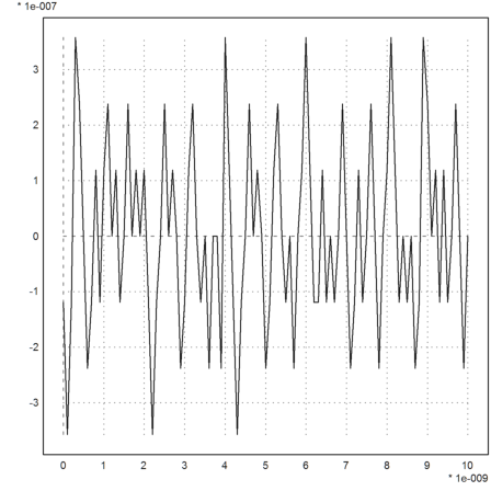
The following example (Rump et al.) is a polynomial, which evaluates very badly.
>p:=[-945804881,1753426039,-1083557822,223200658]; ...
 t:=linspace(1.61801916,1.61801917,100); ...
 plot2d(t-1.61801916,evalpoly(t,p)):

As we see, the plot is completely wrong. Euler can compute a very accurate evaluation using a residuum iteration. This works, since the evaluation of a polynomial can be rewritten as a linear system.
>plot2d(t-1.61801916,xevalpoly(t,p,eps=1e-17)):

For two dimensional problems, Euler has some functions and methods to find guaranteed inclusions.
Let us start with the following example. We wish to solve
![]()
>expr1 &= x*sin(y)-y*cos(x)-5; expr2 &= x^2+cos(y)-8;
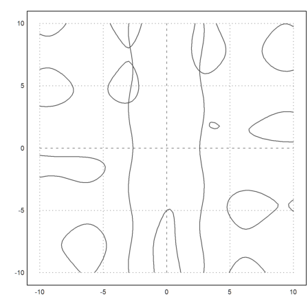
First of all, we can plot an image of the zero sets of both functions.
>plot2d(expr1,level=0,a=-10,b=10,c=-10,d=10,n=80); ...
 plot2d(expr2,level=0,color=2,add=1):

In this example, we can solve one equation first.
>:: solve(expr2,x)
[x = - sqrt(8 - cos(y)), x = sqrt(8 - cos(y))]
Then insert one of the solutions into the other.
>&at(expr1,solve(expr2,x)[2])
- y cos(sqrt(8 - cos(y))) + sqrt(8 - cos(y)) sin(y) - 5
Now solve for y.
>sy:=bisect(&subst(x,y,at(expr1,solve(expr2,x)[2])),6,8)
6.13171103227
Now we can also find an inclusion for this using the interval Newton method.
>syi:=mxminewton(&subst(x,y,at(expr1,solve(expr2,x)[2])),~6.1,6.2~)
~6.131711032268751,6.131711032268759~
Substitute this y back into the formula for x.
>sxi:=&"rhs(solve(expr2,x)[2])"(y=syi)
~2.647914331962739,2.647914331962741~
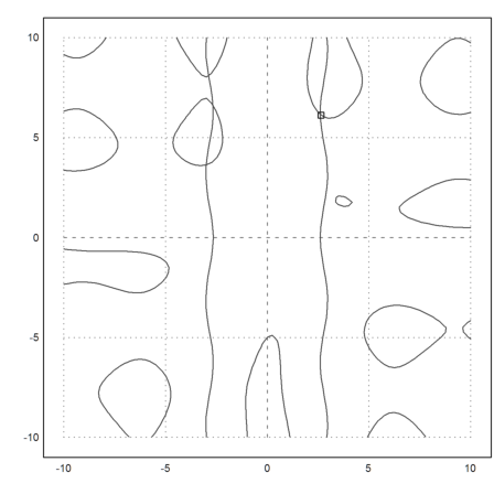
We add this point to our plot.
>plot2d(middle(sxi),middle(syi),points=1,style="[]",add=1):

Euler has also a higher dimensional Newton method. There is a service function for two dimensional problems in x and y. It uses Maxima to compute the partial derivatives.
>mxmnewtonfxy(expr1,expr2,[2.5,6])
[2.64791, 6.13171]
The higher dimensional interval Newton method uses functions. So we define the functions for it. First the function f.
>function f([x,y]) &= [expr1,expr2]
                                                  2
              [x sin(y) - cos(x) y - 5, cos(y) + x  - 8]
Likewise a function for the Jocobian matrix of f.
>function df([x,y]) &= jacobian(f(x,y),[x,y])
               [ sin(y) + sin(x) y  x cos(y) - cos(x) ]
               [                                      ]
               [        2 x             - sin(y)      ]
The multi-dimensional interval Newton method returns an interval inclusion plus a flag. The flag is 1, if the inclusion is a guaranteed inclusion.
>{res,valid}:=inewton2("f","df",[~2.6,2.7~,~6.1,6.2~]); res,
[ ~2.647914331962738,2.647914331962742~,
~6.131711032268749,6.13171103226876~ ]
>valid
1
For two dimensions, there is a general interval method, splitting the area into small rectangles. It returns a list of possible intervals. Everything outside this list is guaranteed not to contain a zero.
We print only the midpoints of the intervals.
>res:=mxmibisectfxy(expr1,expr2,~-10,10~,~-10,10~,0.01); middle(res)
      -2.9834        3.6377
     -2.66113       6.61621
     -2.66113       6.62598
     -2.65137       6.58691
     -2.65137       6.59668
     -2.65137       6.60645
     -2.86621       8.09082
      2.65137       6.12793
      2.65137        6.1377
We can use any of this as a starting point for the interval Newton method and keep only those, which are guaranteed inclusions (maybe loosing some).
>function test(res) ...
 h=[];
 loop 1 to rows(res)
 {y,valid}=inewton2("f","df",res[#]);
 if valid then h=h_y; endif;
 end
 return h
 endfunction
>r:=test(res)
Interval 4 x 2 matrix

~-2.9800345111787907,-2.9800345111787876~     ...
 ~-2.655428339950558,-2.6554283399505545~     ...
~-2.8692456081316013,-2.8692456081315973~     ...
  ~2.6479143319627383,2.6479143319627418~     ...
Then add these points to the plot.
>h:=middle(r)'; plot2d(h[1],h[2],points=1,add=1,style="[]"):
